So now that we survived our crash course on supervised learning, you know the deal — algorithms get a cheat sheet (aka labeled data) and they start flexing on us with their insights.
Today, let’s give love to the real MVPs of the ML supervising world: the actual algorithms themselves.
Specifically, today’s star is one with a straightforward and simple personality: Linear Regression.

Linear Regression. The weirdly correct over-simplifier.
This guy’s entire personality is drawing the best possible straight line through your data and saying “See? I told you I’m right.”
You could say Mr. Regression is an oversimplifier…but somehow, he’s usually right.
Let’s get into it.

📈 Linear Regression - “The Straight Shooter”
Linear Regression is like the simplest form of machine learning. At it’s core, it’s trying to answer this question:
“Can I draw a straight line that best fits this data?”
Imagine a bunch of dots on a graph — each one representing how much someone studied for an exam vs what grade they got.
Linear Regression tries to draw the best straight line through those dots, so you can predict future grades based on hours studied.

Linear Regression: Because apparently, studying does pay off. Who knew?
Linear Regression models the relationship between something called a dependent variable and one or more independent variables, by fitting the linear equation to the observed data.
Independent Variable is what you control or change — it’s the cause.
Dependent Variable is what you measure — it’s the effect.
In the graph above, which do you think is the independent and dependent variables?
That’s correct (I’ll kindly assume you answered it right), our hours studied is the independent variable, and the exam score is the dependent variable.
The result (dependent variable) depends on how much you studied (independent variable).

🧠 The Math Of Linear Regression
Slope-Intercept Form
Linear Regression uses this classic formula from algebra, that you may recognize:
y = mx + b
That’s right! The math behind this fundamental ML algorithm is the Slope Intercept Form equation you learned, probably in 8th grade! It’s quite the superstar in mathematics because it neatly describes any straight line on a graph.
Just in case your memory’s hazy:
y = the thing you’re trying to predict. This is your dependent variable. (e.g exam score)
x = your input. This is your independent variable. (e.g hours studied)
m = the slope of the line. (how much y changes when x changes)
b = the y-intercept. It’s the specific point where your line crosses the vertical y-axis. (the value of y when x is 0)
Your goal is to find the best m (slope) and b (y-intercept)that make your line fit the data as closely as possible.
For example, let’s say our regression line, following y = mx + b, is:
Exam Score = 5 x (Hours Studied) + 50
Here the slope (m) is 5. This means for every 1 extra hour you study, your exam score goes up by 5 points. So if you studied 2 hours, your predicted score is:
5 × 2 + 50 = 50
The slope literally tells you how much studying pays off!
The Loss Function
To find the best line, we need a way to measure how bad our guesses are. Enter the Loss Function.
In the world of ML, a loss function (sometimes called a “cost function”), is simply a mathematical way to measure how “wrong” our models’ predictions are compared to the actual correct answers.
Think of it like this:
Your model makes a guess.
You know what the real answer should have been.
The loss function calculates a single number that tells you exactly “how much” your model messed up.
Obviously, you can see why this is important. Without knowing the level error, you wouldn’t be able to “train” your model to improve.
Okay, heads up. I’m about to throw a weird-looking equation at you, but fret not, because I’ll break it down. Introducing MSE (Mean Squared Error):

Translating the above to plain English: “Your predictions suck bro.”
MSE is the brains commonly used behind the loss function. Despite how it looks, what it calculates is actually quite simple: how far off the model’s guess was.
The goal of training is to make the MSE as small as possible — smaller means our predictions are closer to the actual answers.
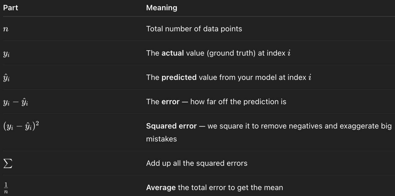
Here’s breaking down each part of the equation:

Basically, this equation finds the difference between each real and predicted value, squares those differences, adds them up, and divides by the number of points to get the average error.
Example. Let’s say your actual exam scores were [70, 80, 90]. Now, let’s say your model predicted [75, 78, 85].
According to MSE, the errors were:
(70–75)² = 25
(80–78)² = 4
(90–85)² = 25
So plugging those errors into the equation we get the following:


Conclusion
Linear Regression is like the “Hello World” of machine learning — simple, smart, and great for predictions.
It fits the best line through your data using y = mx + b, and checks how far off it is with Mean Squared Error (MSE) — squaring the errors and averaging them. The smaller the MSE, the better the model!
And that wraps up our first performer: Linear Regression! What did you think?
Stay tuned — next up, things get curvy with Logistic Regression!

